Artistic Style

在艺术领域，我们已经掌握了采用不同的内容和风格创造别具一格的图画。虽然我们并不知道算法如何才能实现图画创造，但是在图像识别领域深度网络的实现给了我们希望。下面我们就介绍一种基于深度网络实现的高质量艺术图像生成技术。这个系统用网络拆分和合并图片的内容和形式，通过组合创造新图片。同时我们的工作也可以帮助理解人类的艺术创造。

DNN

深度神经网络用于处理图片已经深入开发，其中最强大的一个算法就是CNN，CNN包罗了很多层的小计算单元，逐层地处理图片的信息。每一层的单元可以理解为图片filter的集合，每一个filter都能从图片中提取相应的特征，所以某一层的输出我们叫它 feature maps：differently filtered versions of the input image.

Content representation

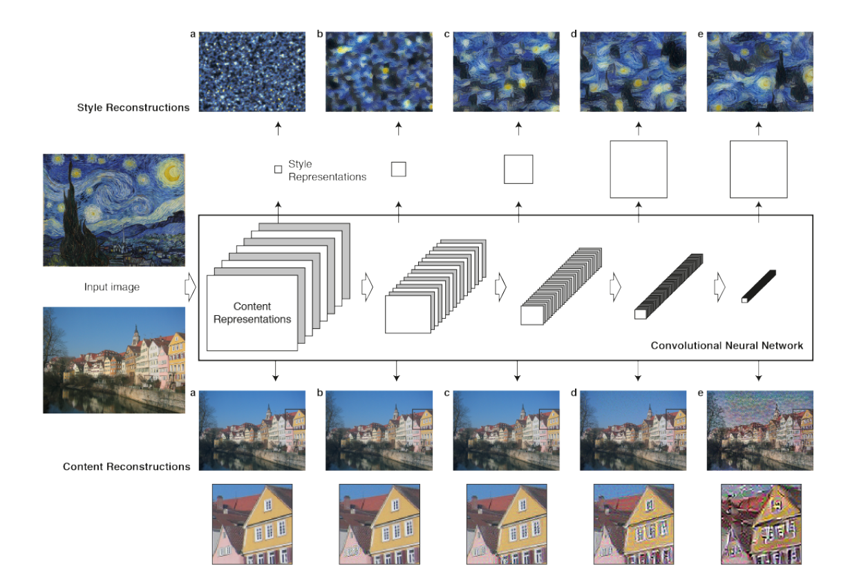
当CNN网络用于图片识别的时候，它每一层都在不断提取更高层次的特征，使图片的表征越来越显性。换句话说，沿着网络的深入方向，原始的图片表现越来越关注图片的实际内容而不是像素的细节。我们可以通过图片重构得到每一层的图片信息(方法见后面)。更高层的网络抓住了图片的hign-level content in terms of objects and their arrangement in the origin image 但是并不表征每一个确定的像素信息。而低层的表征仅仅是重新生成了原始图片的像素信息。所以我们将高层的feature responses 称为content representation

Style representation

为了得到原始图片的风格表征，我们使用了一个特征空间，这个空间被设计来capture texture information. 这个特征空间建立于每一层的filter responses 之上，它包含了correlations between the different filter responses over the spatial extent of the feature maps(See Methods). 通过引入不同layers的相关性(correlations)，我们获得了一个静止的、多维度的原始图片表征，它展现了图片的纹理特征(texture information)而不是全局的分布。再一次，我们可以通过重构图片that matches the style representation of a given input image by these style feature spaces build on different layers of the network. 实际上，我们从style feature重构得到的图片反映了原始图片纹理的特征，保留了原始图片的颜色和局部的结构。更进一步的，随着网络的深入，特征的数量和复杂度也在加深，我们可以用很多层的style feature 来表征图片的风格。我们称这种多维度的表达为style representation

Explanation

这篇文章的核心发现就是: The representations of content and style in the CNN are separable. 也就是说，我们可以分别操作两种表达特征来生成新的、从感觉上有意义的图片。为了演示这个发现，我们将两个不同图片的内容和风格混合，如下图：

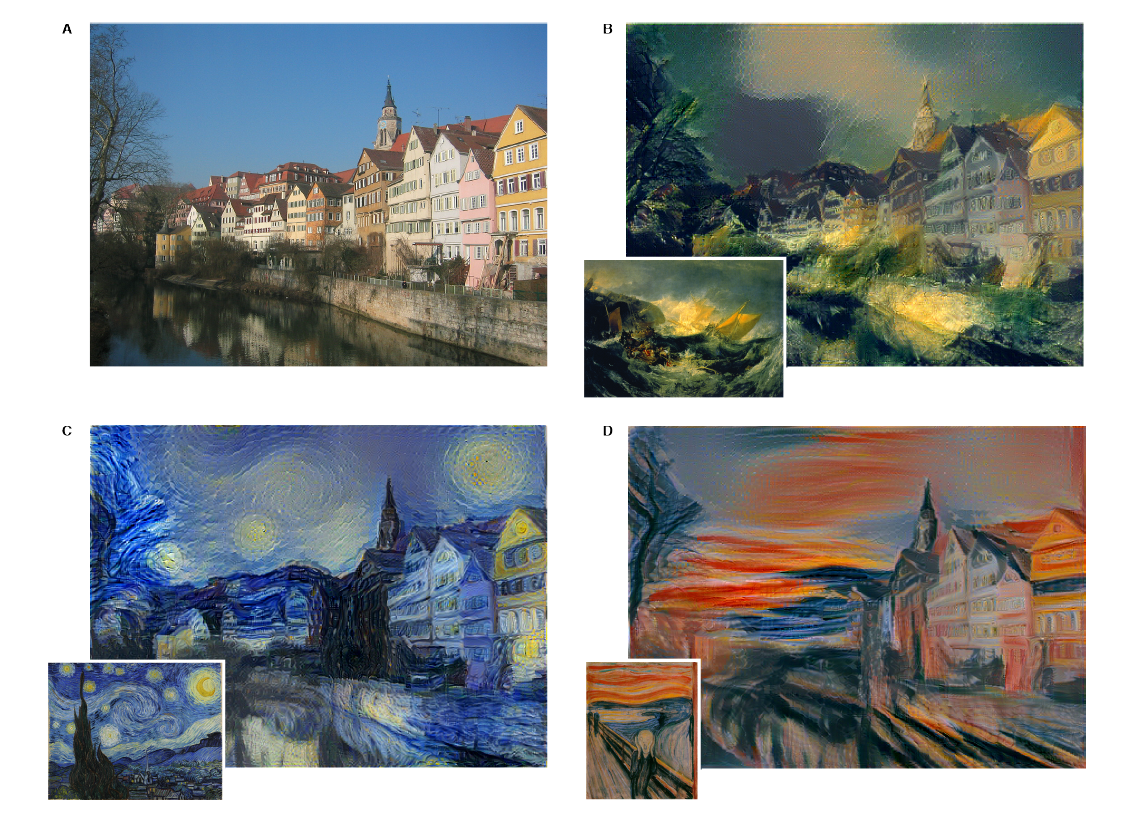
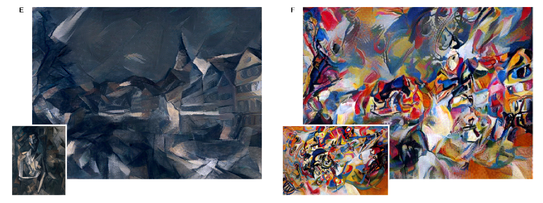
(注：we matched the content representation on layer ‘conv4_2’ and the style representations on layers ‘conv1_1’,’conv2_1’,’conv3_1’,’conv4_1’ and ‘conv5_1’, $w_l=1/5$ in those layers, the ratio $\alpha/\beta$ was either $1\times 10^{-3}$ on B,C,D and $1\times 10^{-4}$ on E,F )

这些图片通过综合性的找到一幅图片同时匹配摄影图片的内容表达和艺术作品的风格表达(simultaneously matches the content representation of the photograph and the style representation of the respective piece of art). 原始图片全局的分布被保留下来，而颜色和风格混合了艺术作品，就好像艺术家的作品一样。前面也提到，the style representation 是多层次的表述(includes multiple layers of the neural network). Style can also be defined more locally by including only a smaller number of lower layers, 能得到不同视觉体验。当我们匹配高层的风格特征时候，图片的局部特征会在更大的维度得到匹配，这样形成的视觉体验会更加光滑和连续，所以最逼真的图片经常都是通过最高层的风格特征重构的。下图展示了通过不同层数重构的图片(横轴表示不同的混合参数)：

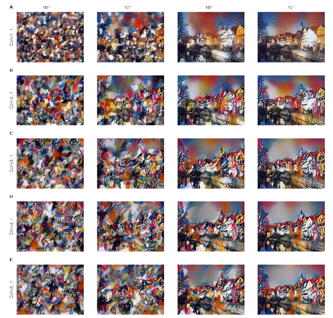
当然，图片的内心和风格不能被完整分离，当合成不同图片来源的内容和风格时候，基本不可能存在一张图片能完美地匹配两者的限制。但是，我们定义的损失函数包含了内容匹配和风格匹配两个部分，它们是相互分开的。所以我们可以定义两部分的权重，就如上图展示的一样，当我们强调风格的时候，生成的图片会更加偏向于原始的艺术图片，很难清晰地看到摄影图片的内容；而我们更加注重内容的时候，虽然可以清晰看到摄影图片的内容，但是风格匹配被弱化了。我们可以调整中间的系数让图片看起来更加符合我们的预期。

Conclusion

我们展示了一个人工的神经网络用于将图片的内容和风格分开，实现了重组图片的可能。我们通过摄影的图片和艺术家的作品混合演示了这个可能性。特别的，In particular,we derive the neural representations for the content and style of an image from the feature responses of high performing DNN trained on object recognition(网络是训练好的，训练的目标是图片识别，其实这个网络只是为了能够反映原始的图片特征即可，所以以图片识别为训练目标也不错，另外鄙人认为图片自编码的方法也是很不错的，而且不用标记图片). 据我们所知，这是第一次将图片的内容和风格分开的实现。 Features from Deep Neural Networks trained on object recognition have been previously used for style recognition in order to classify artworks according to the period in which they were created. 在这个前人工作中，分类器是基于高层的特征空间建立的，也就是我们说的content representations. 我推测将其转换为静止的特征空间(就像我们的style representation)可能会获得更好的风格分类结果。我相信我们的思想会在很多图片领域得到应用。Importantly, the mathematical form of our style representations generates a clear, testable hypothesis(假设) about the representation of image appearance down to the single neuron level. 我们的风格表述仅仅简单地计算不同网络单元的相关性，具有简洁性和有效性。为什么我们的网络可以自动学习image representations that allow the separation of image content from style? 可能的解释是：当网络学习物体识别的时候，网络必须具有图片扰动保持性(the network has to become invariant to all image variation that preserves object identity). Representations that factorise the variation in the content of an image and the variation in its appearance would be extremely practical for this task. Thus, our ability to abstract content from style and therefore our ability to create and enjoy art might be primarily a preeminent(卓越的) signature of the powerful inference capabilities of our visual system.

Methods

文中提到的识别网络结构为VGG-Network，我们使用了一个特征空间provided by the 16 convolutional and 5 pooling layers of the 19 layer VGG network. 我们不使用任何全连接层。对于图片合成，我们发现使用平均池化比最大池化好(slightly more appealing)，这就是为什么我们使用平均池化。每一次的网络都设计了非线性的filter，随着网络的深入复杂度在上升。这样，一个输入的图片$\vec{x}$ is encoded in each layer of the CNN by the filter responses to that image. 一层网络with $N_l$ 不同的filters 有$N_l$ feature maps each of size $M_l$ , 其中$M_l$ 是feature map的高度乘以宽度。所以第$l$ 层的responses 可以被存储为一个矩阵$F^l\in R^{N_l\times M_l}$ where $F_{ij}^l$ is the activation of the $i^{th}$ filter at position j in layer $l$. 为了看到不同层编码的图片信息，我们在一张白噪音的图片上使用梯度下降法(content reconstructions)，找到一张图片使其feature responses和原始的图片相匹配。 So let $\vec{p}$ and $\vec{x}$ be the original image and the image that is generated and $P^l$ and $F^l$ their respective feature representation in layer $l$. 我们定于如下的平方误差：

$L_{content}(\vec{p},\vec{x},l)=\frac{1}{2}\sum_{i,j}(F_{ij}^l-P_{ij}^l)^2$

这个loss关于activations in layer $l$ 的导数为：

$\frac{\partial L_{content}}{\partial F_{ij}^l}=(F^l-P^l)_{ij}\quad if\; F_{ij}>0\quad else\quad 0$

因为采用Relu输出，所以不存在小于0的部分。从这导数开始，关于$\vec{x}$ 的导数可通过标准的BP算法计算，所以我们不断调整$\vec{x}$ 直到它产生了一样的response in a certain layer of CNN as the original image $\vec{p}$ .

在每一层CNN response的上面我们还生成了一个style representation that computes correlations between the different filter responses, where the expectation is taken over the spatial extend of the input image. 这些特征的相关性是通过Gram矩阵表现的 $G^l\in R^{N_l\times N_l}$ ,where $G_{ij}^l$ is the inner product between the vectorised feature map i and j in layer $l$ :

$G_{ij}^l=\sum_k F_{ik}^l F_{jk}^l$

为了生成一个匹配给定图片风格的纹理(style reconstructions)，我们在一张白噪音的图片上使用梯度下降法，来找到一张图片matches the style representation of the original image. This is done by minimizing the mean-squared distance between the entries of the Gram matrix from the original image and the Gram matrix of the image to be generated. So let $\vec{a}$ and $\vec{x}$ be the original image and the image that is generated and $A^l$ and $G^l$ their respective style representations in layer $l$ . 损失函数定义为：

$E_l=\frac{1}{4N_l^2 M_l^2}\sum_{i,j} (G_{ij}^l-A_{ij}^l)^2$

总共的损失函数为：

$L_{style}(\vec{a},\vec{x})=\sum_{l=0}^L w_l E_l$

其中$w_l$ 表示了每一层对于total loss的权重。$E_l$ 关于activations in layer l 的导数为：

$\frac{\partial E_l}{\partial F_{ij}^l}=\frac{1}{N_l^2 M_l^2}((F^l)^T(G^l-A^l))_{ji}\quad if\; F_{ij}^l>0 \quad else \quad 0$

$E_l$ 关于更低层的输出的导数可以快速通过BP算法实现，上面第一幅图的style reconstructions base on layer (a)’conv1_1’,(b)’conv1_1’ and ‘conv2_1’ ,(c)’conv1_1’,’conv2_1’ and ‘conv3_1’,(d)’conv1_1’,’conv2_1’,’conv3_1’ and ‘conv4_1’ ,(e)’conv1_1’,’conv2_1’,’conv3_1’,’conv4_1’ and ‘conv5_1’.

为了混合一张摄影的内容和一张绘画的风格，我们联合了两个目标函数，from the content representation of the photograph in one layer of the network and the style representation of the painting in a number of layers of the CNN. So let $\vec{p}$ be the photograph and $\vec{a}$ be the artwork.整体的损失函数为：

$L_{total}(\vec{p},\vec{a},\vec{x})=\alpha L_{content}(\vec{p},\vec{x})+\beta L_{style}(\vec{a},\vec{x})$

其中$\alpha\;and\;\beta$ 是内容与风格间的权衡系数。

Extend

首先鄙人认为这个原始的网络训练方法可以尝试通过自编码实现。主要是为了降低人工的标记工作，当然我们如果可以的话可以通过已有的识别网络标记。其次，可能在内容分离方面由于原始图片还带有其自己的色彩和风格，所以有一定影响，可以尝试替换目标损失函数为：

$L_{total}(\vec{p},\vec{a},\vec{x})=\alpha L_{content}(\vec{p},\vec{x})+\beta L_{style}(\vec{a},\vec{x})-\gamma L_{style}(\vec{p},\vec{x})$

当然，由于style分离也不是很完全，所以$\gamma$ 参数要设置得很小很小，作用不大，此处写出来是为了提出这样一个思想，扩展一下。

捎带介绍一下VGG-Network，其实这就是一个简单的CNN网络，只是把大的卷积核拆分为多个3x3的卷积核，一个简单的网络代码如下：

def conv_op(input_op,name,kh,kw,n_out,dh,dw,p):
	n_in=input_op.get_shape()[-1].value
	with tf.name_scope(name) as scope:
		kernel=tf.get_variable(scope+'w',shape=[kh,kw,n_in,n_out],dtype=tf.float32,
			initializer=tf.contrib.layers.xavier_initializer_conv2d())
		conv=tf.nn.conv2d(input_op, kernel, strides=[1,dh,dw,1], padding='SAME')
		bias=tf.Variable(tf.constant(0.0,shape=[n_out],dtype=tf.float32),trainable=True,name='bias')
		z=tf.nn.bias_add(conv, bias)
		activation=tf.nn.relu(z,name=scope)
		p+=[kernel,bias]
		return activation

def fc_op(input_op,name,n_out,p):
	n_in=input_op.get_shape()[-1].value
	with tf.name_scope(name) as scope:
		w=tf.get_variable(scope+'w',shape=[n_in,n_out],dtype=tf.float32,
			initializer=tf.contrib.layers.xavier_initializer())
		bias=tf.Variable(tf.constant(0.1,dtype=tf.float32,shape=[n_out]),trainable=True,name='bias')
		activation=tf.nn.relu_layer(input_op, w, bias)
		p+=[w,bias]
		return activation

def maxpool_op(input_op,name,kh,kw,dh,dw):
	return tf.nn.max_pool(input_op, [1,kh,kw,1], strides=[1,dh,dw,1], padding='SAME',name=name)

def inference_op(input_op,keep_prob):
	p=[]
	conv1_1=conv_op(input_op, 'conv1_1', 3, 3, 64, 1, 1, p)
	conv1_2=conv_op(conv1_1, 'conv1_2', 3, 3, 64, 1, 1, p)
	pool1=maxpool_op(conv1_2, 'pool1', 2, 2, 2, 2)

	conv2_1=conv_op(pool1, 'conv2_1', 3, 3, 128, 1, 1, p)
	conv2_2=conv_op(conv2_1, 'conv2_2', 3, 3, 128, 1, 1, p)
	pool2=maxpool_op(conv2_2, 'pool2', 2, 2, 2, 2)

	conv3_1=conv_op(pool2, 'conv3_1', 3, 3, 256, 1, 1, p)
	conv3_2=conv_op(conv3_1, 'conv3_2', 3, 3, 256, 1, 1, p)
	conv3_3=conv_op(conv3_2, 'conv3_3', 3, 3, 256, 1, 1, p)
	pool3=maxpool_op(conv3_3, 'pool3', 2, 2, 2, 2)

	conv4_1=conv_op(pool3, 'conv4_1', 3, 3, 512, 1, 1, p)
	conv4_2=conv_op(conv4_1, 'conv4_2', 3, 3, 512, 1, 1, p)
	conv4_3=conv_op(conv4_2, 'conv4_3', 3, 3, 512, 1, 1, p)
	pool4=maxpool_op(conv4_3, 'pool4', 2, 2, 2, 2)

	conv5_1=conv_op(pool4, 'conv5_1', 3, 3, 512, 1, 1, p)
	conv5_2=conv_op(conv5_1, 'conv5_2', 3, 3, 512, 1, 1, p)
	conv5_3=conv_op(conv5_2, 'conv5_3', 3, 3, 512, 1, 1, p)
	pool5=maxpool_op(conv5_3, 'pool5', 2, 2, 2, 2)

	shp=pool5.get_shape()
	flatten_shape=shp[1].value*shp[2].value*shp[3].value
	resh1=tf.reshape(pool5, shape=[-1,flatten_shape], name='resh1')

	fc6=fc_op(resh1, 'fc6', 4096, p)
	fc6_drop=tf.nn.dropout(fc6, keep_prob=keep_prob,name='fc6_drop')

	fc7=fc_op(fc6_drop, 'fc7', 4096, p)
	fc7_drop=tf.nn.dropout(fc7, keep_prob,name='fc7_drop')

	fc8=fc_op(fc7_drop,	'fc8', 1000, p)
	softmax=tf.nn.softmax(fc8)
	prediction=tf.argmax(softmax,1)
	return prediction,softmax,fc8,p

这里的代码例子还包括了全连接层，另外pooling的方法本文采用的是平均池化，这个要注意。

Blog