中国围棋博大精深，听说想要用穷举法搜索它的整个空间可以用完地球的所有原子来计数。这么一个复杂的任务，多少年来我们认为只有人类才可以掌握围棋的真谛，而要想实现一个能与人类对抗的围棋算法，现在还是太早了。可是让人大跌眼镜的是Google DeepMind 居然造就了一代AlphaGo，打败了人类顶尖的围棋选手，而就在不久前，听说新一代Alpha Zero再创辉煌，在没有人类的经验学习下大败初代AlphaGo。一石激起千层浪，究竟是什么神奇的力量在掌握着AlphaGo？今天，我们走近初代AlphaGo。

很多的游戏理论上都有一个最佳的价值函数 $v^\ast(s)$ ，它可以在任何一个状态s下断言游戏的结果，只要后面游戏的双方都按照最佳的操作完成比赛。这类游戏可以通过递归计算出这个最佳的价值函数，而这个递归的树结构有$b^d$ 这么多行动序列，其中b是游戏的广度（每一个状态下合法的移动数），d是游戏的长度。显然对于围棋这样一个庞大的游戏来说，穷举是不可行的，但是可以通过以下两个主要的策略来构建有效的搜索空间：1 搜索的深度可以通过状态价值估计（Position evaluation）减少，在状态s的时候截断搜索树，而状态s下的子树可以通过状态估计函数 $v(s)=v^\ast(s)$预测结果。2 搜索的宽度可以通过服从一定动作策略的动作随机数替代(the breadth of the search may be reduced by sampling actions from a policy $p(a\mid s)$ that is a probability distribution over possible moves a in position s)。

我们设计AlphaGo 就是通过深度卷积网络来减少搜索树的广度和深度：evaluating positions using a value network, and sampling actions using a policy network。我们首先从一个监督学习开始: raining a supervised learning (SL) policy network $p_σ$ directly from expert human moves，我们也训练了一个快速下子的网络：we also train a fast policy $p_π$ that can rapidly sample actions during rollouts，接着我们训练一个增强学习的网络：train a reinforcement learning (RL) policy network $p_ρ$ that improves the SL policy network by optimizing the final outcome of games of self play，最后我们通过增强学习的网络构建了一个价值估计函数：we train a value network $v_θ$ that predicts the winner of games played by the RL policy network against itself。总的结构如下图：

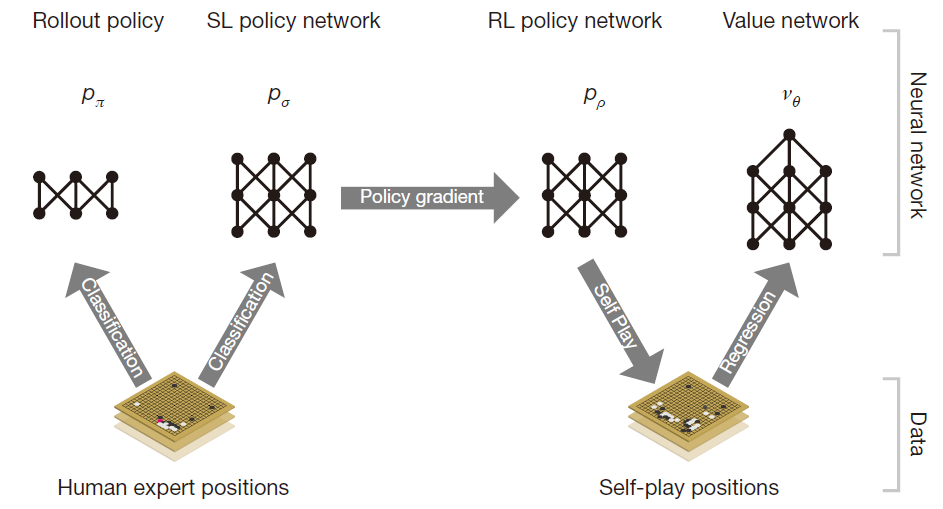
SL Policy network $p_σ$

训练集来自人类高手的对局记录，通过随机采样和梯度下降来最大化极大似然估计：

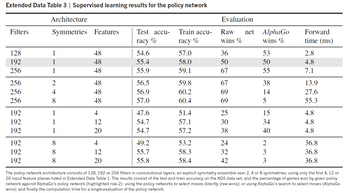
其中激活层采用softmax。我们通过训练13层的策略网络，在测试集上实现了57.0%的正确性。其它一些研究团队只能达到44.4%的准确度，而准确度微小的改进就可以很大地促进策略的有效性（Small improvements in accuracy led to large improvements in playing strength ）：

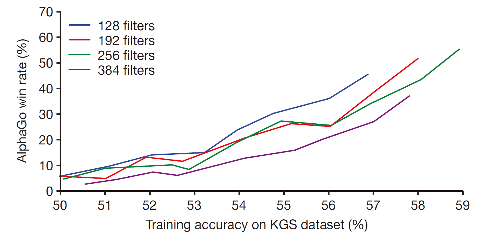
Plot showing the playing strength of policy networks as a function of their training accuracy. Policy networks with 128, 192, 256 and 384 convolutional filters per layer were evaluated periodically during training; the plot shows the winning rate of AlphaGo using that policy network against the match version of AlphaGo

We also trained a faster but less accurate rollout policy $p_π(a\mid s)$, using a linear softmax of small pattern features with weights π; this achieved an accuracy of 24.2%, using just 2 μs to select an action, rather than 3 ms for the policy network.

RL Policy network $p_\rho$

RL 策略网络采用SL一样的结构，这样就可以用SL的参数初始化RL的参数，即 $\rho=\sigma$. 我们让现在的策略网络 $p_\rho$ 同一个随机选择的前代 $p_\rho-$ 对弈。其中的reward function r(s) 是这样的定义的：对于不是最终的time steps, 回报为0，对于最终time steps T: $z_t=\pm r(S_T)$ 就是最后的reward，正负号是相对现在的选手来说的：赢家是+1，输的一方是-1。然后我们就可以根据最后的回报利用随机梯度下降更新参数：

我们测试RL策略网络的效果，通过动作采样 $a_t \sim p_\rho(·\mid s_t)$ ，RL网络在80%的情况下可以战胜SL网络。

RL value networks

位置价值估计$v^p(s)$ 预测状态s的结果通过双方采取同样的策略p:

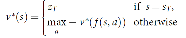
我们希望得到最佳的价值近似 v*(s); 但是实际我们只能得到我们的最强近似$v^{p_\rho}(s)$, 使用增强学习策略网络$p_\rho$ . We approximate the value function using a value network $v_θ(s)$ with weights $\theta$ ：$v_\theta(s) \approx v^{p_\rho}(s) \approx v^\ast(s)$ ,We train the weights of the value network by regression on state-outcome pairs (s, z), using stochastic gradient descent to minimize the mean squared error (MSE) between the predicted value $v_θ(s)$, and the corresponding outcome z :

这些数据是通过RL policy自我对弈得到的，但是我们发现连续的下子是十分关联的，这样训练很可能会过拟合。所以我们仿照SL先建立一个记忆库，然后随机抽样训练。Training on this data set led to MSEs of 0.226 and 0.234 on the training and test set respectively, indicating minimal overfitting.训练的有效性比较还可以见下图，可以看出value function比快速下子策略更准确，并且接近RL policy，而花费远远更少的计算：

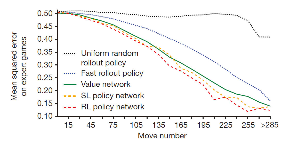
横坐标是表示已经下过的步数，其它的四个策略都是通过100次迭代的平均结果来计算的。

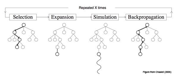
MCTS algorithm

搜索树包括四个阶段，先看图：

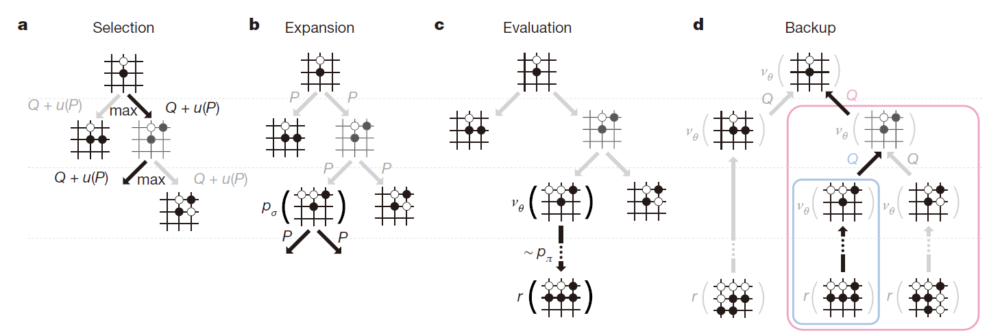
在根节点处要选择下一步的动作的时候，其中每一个节点(s,a) stores an action value Q(s, a), visit count N(s, a), and prior probability P(s, a)：

先扩展L步，每一步($t\le L$)的扩展选择的原则是：

so as to maximize action value plus a bonus that is proportional to the prior probability but decays with repeated visits to encourage exploration：

如果第L步的时候满足$N(s_T,a)>n_{tr}$ ,则扩展该节点到L+1步，利用SL policy初始化L+1步所有节点（合法的action a）的先验概率$P(s,a)=p_\sigma(a\mid s)$ 。

然后最后选择的一个节点（设为$s_L$）有两种评估方法：第一种是通过价值网络$v_\theta(s_L)$ ，第二种是通过通过快速走子策略获取最后的outcome $z_L$ 。两种评估方法做耦合，参数为$\lambda$ ，得到一个叶子节点的评估价值$V(s_L)$

最后，所有经过的节点参数更新，N(s,a)需要加1，Q(s,a)则取所有经过此节点的评估平均：

where $s_L^i$ is the leaf node from the ith simulation, and 1(s, a, i) indicates whether an edge (s, a) was traversed during the ith simulation.

重复以上步骤n次（比如说取n=10000），然后选择根节点出发访问次数最多的子节点作为下一步的落子。

很奇怪的是我们为什么要选择SL policy来生成先验概率而不是用RL policy，这是因为RL policy选择的动作比较集中，探索性不足效果没有SL policy好，但是通过RL policy训练的价值网络的确比SL policy训练的价值网络好，也说明了RL policy的高效性。

由于MSTS计算复杂度比一般的策略大幅上升，所以我们需要进行分布式和多线程的计算。另外一张解释MCTS的图或许更加清晰，如图：

Evaluating the playing strength

打败了所有已有的围棋算法，并且也击败了人类棋手。我们发现在选择评价函数的时候有两条路径，通过参数$\lambda$ 控制，综合下来得到参数取值0.5的时候最好：这也说明了value network和rollout policy的互补性。多个策略的重要性可以通过以下图表示：

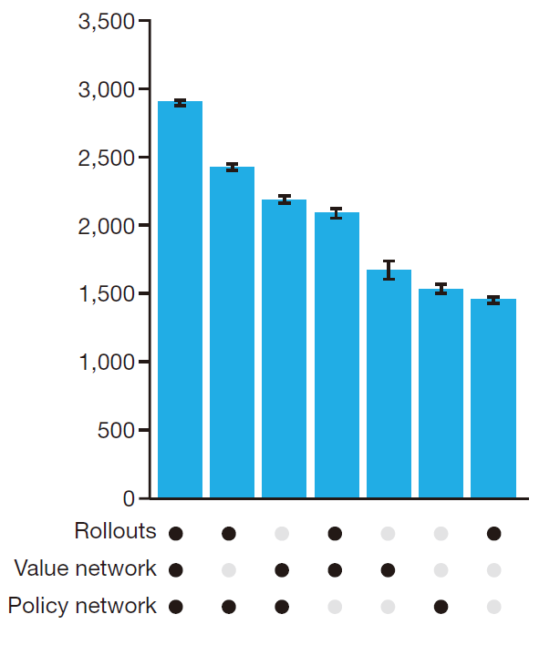
Programs were evaluated on an Elo scale: a 230 point gap corresponds to a 79% probability of winning, which roughly corresponds to one amateur dan rank advantage on KGS.

Methods

前面介绍了大致的主要算法，但是一些细节并不明确，所以这里详细解读算法：

Problem setting

围棋是一类交替马尔科夫游戏（alternating Markov games），这类游戏有以下特征：a state space S (where state includes an indication of the current player to play); an action space A(s) defining the legal actions in any given state s ∈ S; a state transition function f(s, a, ξ) defining the successor state after selecting action a in state s and random input ξ (for example, dice); and finally a reward function $r_i(s)$ describing the reward received by player i in state s。而更加特殊的围棋是一个双玩家零合的游戏（two-player zero-sum games），$r^1(s)=-r^2(s)=r(s)$ ，其状态价值函数也有以下性质：

Prior work

Depth-first minimax search with alpha–beta pruning has achieved superhuman performance in chess, checkers and Othello, but it has not been effective in Go. Temporal-difference learning(通过TD-error 学习，TD-error的应用使我们每一步都可以进行训练，而不需要等一个episode结束才可以获得每个状态的目标价值) has also been used to train a neural network to approximate the optimal value function, achieving superhuman performance in backgammon.

先前的工作都是手动设计features,而我们AlphaGo通过深度神经网络自主学习，获得更高效的feature。另外我们利用MCTS开辟了另外一种方法：AlphaGo’s use of value functions is based on truncated Monte Carlo search algorithms, which terminate rollouts before the end of the game and use a value function in place of the terminal reward. AlphaGo’s position evaluation mixes full rollouts with truncated rollouts, resembling in some respects the well-known temporal-difference learning algorithm TD(λ).

Search algorithm

我们的算法总称：asynchronous policy and value MCTS algorithm (APV-MCTS). Each node s in the search tree contains edges (s, a) for all legal actions a ∈ A(s). Each edge stores a set of statistics,

其中P(s,a)是先验概率，$W_v(s,a),W_r(s,a)$ 分别是通过价值函数和rollout策略得到的通过节点（s,a）的价值总和，$N_v(s,a),N_r(s,a)$ 是对应的通过次数(理论上是同一个，但是分为两个可以方便中间某些操作)。Q(s,a)就是综合的该节点的动作价值（the combined mean action value）。

Selection

The first in-tree phase of each simulation begins at the root of the search tree and finishes when the simulation reaches a leaf node at time step L(共走L步). At each of these time steps, t < L, an action is selected according to the statistics in the search tree,

where $C_{puct}$ is a constant determining the level of exploration; 一开始会倾向于先验概率更大的分支，后面逐渐倾向于action value更大的分支。$\sqrt{\sum_b N_r(s,b)}$ 表示父节点经过的次数，所以一定是大于1的(我们更新的时候先更新父节点再更新子节点，先更新Nr，再更新u(s,a))。

这里没有提到如何扩展新节点，当一个父节点没有子节点的时候，利用SL policy得到所有其子节点的先验概率，初始化如下：$u(s,a)=P(s,a)=P_\sigma(a\mid s),Q(s,a)=0$ ,所以一开始选择的时候仅仅是按照先验概率来选择的，只有L步扩展和评估完成后才会更新这些参数(u(s,a)其实也是保存的，这样方便编程，初始化为先验概率就是为了方便第一次选择)。

Evaluation

The leaf position $s_L$ is added to a queue for evaluation $v_\theta(s_L)$ by the value network, unless it has previously been evaluated. The second rollout phase of each simulation begins at leaf node $s_L$and continues until the end of the game. At each of these time-steps, t ≥ L, actions are selected by both players according to the rollout policy, $a_t\sim p_\sigma(·\mid s_t)$

Backup

在探索结束前的每一步 (step t ≤ L), 对探索经过的节点的统计数据加以修改，假装它输掉了$n_{vl}$ 次比赛, $N_r(s_t,a_t)\gets N_r(s_t,a_t)+n_{vl};W_r(s_t,a_t)\gets W_r(s_t,a_t)-n_{vl}$ ; this virtual loss discourages other threads from simultaneously exploring the identical variation(只有在多线程工作的时候才需要这么做，单线程不需要，因为单线程一次探索完成更新后才进行新的一次，由于中间过程Q是不更新的，所以$W_r(s_t,a_t)$ 更新其实不需要)。当本次探索结束后，the rollout statistics are updated in a backward pass through each step t ≤ L, replacing the virtual losses by the outcome：

异步地，我们更新value estimate 路线：

The overall evaluation of each state action is a weighted average of the Monte Carlo estimates:

一次更新完成之后我们循环n次，多线程我们就循环n/threads number 次数

Expansion

When the visit count exceeds a threshold, $N_r(s,a)>n_{thr}$ , the successor state s′ = f(s, a) is added to the search tree. The new node is initialized as :

哪里来的$\beta$ ，其实我们SL过程采用的softmax输出，有一个softmax temperature 参数，就是它：

The threshold $n_{thr}$is adjusted dynamically to ensure that the rate at which positions are added to the policy queue matches the rate at which the GPUs evaluate the policy network. 简介的说就是调整阈值刚好适应空闲GPU计算的能力。

Action

At the end of search AlphaGo selects the action with maximum visit count(最多访问); this is less sensitive to outliers than maximizing action value. The search tree is reused at subsequent time steps: 选择的子节点成为新的根节点; 新根节点的子节点保留，其余的扔掉，其实这是树结构直接完成的。

AlphaGo resigns（罢工） when its overall evaluation drops below an estimated 10% probability of winning the game, that is, $\underset{a}{max} \; Q(s,a)<-0.8$ 。

Codes

下面是一个Google DeepMind的MCTS代码，可以结合理解：

class TreeNode(object):
    # MCTS tree 节点. 每个节点有自己价值Q,先验概率P,访问次数n_visit等
    def __init__(self, parent, prior_p):
        self._parent = parent
        self._children = {}  # a map from action to TreeNode
        self._n_visits = 0
        self._Q = 0
        #u在第一次调用update的时候更新，初始化这样可以方便第一次选择
        self._u = prior_p
        self._P = prior_p

    def expand(self, action_priors):
        #action_priors 是通过SL policy得到的
        for action, prob in action_priors:
            if action not in self._children:
                self._children[action] = TreeNode(self, prob)

    def select(self):
        #选择最大的Q+u子节点
        return max(self._children.iteritems(), key=lambda act_node: act_node[1].get_value())

    def update(self, leaf_value, c_puct):
        #先更新访问次数
        self._n_visits += 1
        # Update Q ，这个加上变化量和全部取平均是一样的
        self._Q += (leaf_value - self._Q) / self._n_visits
        #如果不是根节点还需要更新u
        if not self.is_root():
            self._u = c_puct * self._P * np.sqrt(self._parent._n_visits) / (1 + self._n_visits)

    def update_recursive(self, leaf_value, c_puct):
        #backup更新，先更新父节点，再更新本身，这样父节点的访问次数一定大于0
        if self._parent:
            self._parent.update_recursive(leaf_value, c_puct)
        self.update(leaf_value, c_puct)

    def get_value(self):
        return self._Q + self._u

    def is_leaf(self):
        #判断是否有叶子，没有则需要扩展
        return self._children == {}

    def is_root(self):
        #判断是不是父节点
        return self._parent is None


class MCTS(object):
    def __init__(self, value_fn, policy_fn, rollout_policy_fn, lmbda=0.5, c_puct=5,
                 rollout_limit=500, playout_depth=20, n_playout=10000):
        #playout_depth就是L，n_playout就是探索总共的次数
        self._root = TreeNode(None, 1.0)
        self._value = value_fn
        self._policy = policy_fn
        self._rollout = rollout_policy_fn
        self._lmbda = lmbda
        self._c_puct = c_puct
        self._rollout_limit = rollout_limit
        self._L = playout_depth
        self._n_playout = n_playout

    def _playout(self, state, leaf_depth):
        #探索，深度是leaf_depth，state是目前的状态一个copy
        node = self._root
        for i in range(leaf_depth):
            # Existing nodes already know their prior.
            if node.is_leaf():
                action_probs = self._policy(state)
                #可能有戏结束了
                if len(action_probs) == 0:
                    break
                #扩展所有子节点
                node.expand(action_probs)
            #选择下一个节点 max:Q+u,第一次选择其实就是max:prior
            action, node = node.select()
            state.do_move(action)

        #更新节点action value
        v = self._value(state) if self._lmbda < 1 else 0
        z = self._evaluate_rollout(state, self._rollout_limit) if self._lmbda > 0 else 0
        leaf_value = (1 - self._lmbda) * v + self._lmbda * z

        #backup
        node.update_recursive(leaf_value, self._c_puct)

    def _evaluate_rollout(self, state, limit):
        #快速走子策略，获得最后的结果返回
        player = state.get_current_player()
        for i in range(limit):
            action_probs = self._rollout(state)
            if len(action_probs) == 0:
                break
            max_action = max(action_probs, key=itemgetter(1))[0]
            state.do_move(max_action)
        else:
            # If no break from the loop, issue a warning.
            print("WARNING: rollout reached move limit")
        winner = state.get_winner()
        if winner == 0:
            return 0
        else:
            return 1 if winner == player else -1

    def get_move(self, state):
        #首先进行 _n_playout这么多次探索
        for n in range(self._n_playout):
            state_copy = state.copy()
            self._playout(state_copy, self._L)
        #下一步选择访问次数最多的子节点
        return max(self._root._children.iteritems(), key=lambda act_node: act_node[1]._n_visits)[0]

    def update_with_move(self, last_move):
        #更新根节点，选择下一个子节点作为新的根节点
        if last_move in self._root._children:
            self._root = self._root._children[last_move]
            self._root._parent = None
        else:
            self._root = TreeNode(None, 1.0)

Rollout policy

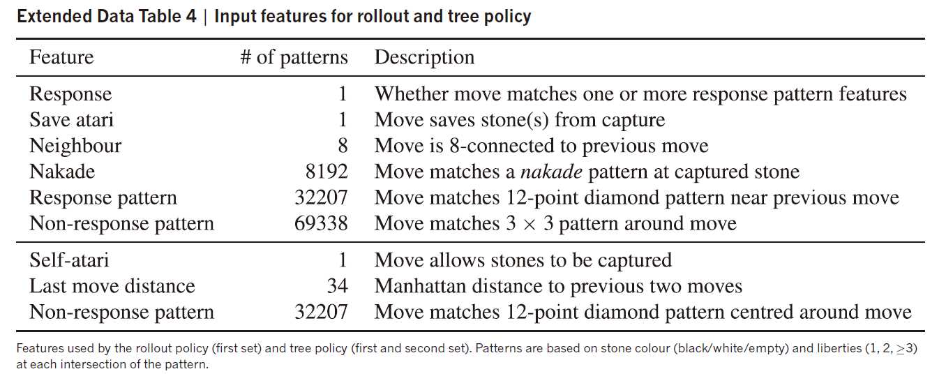
The rollout policy $p_π(a\mid s)$ is a linear softmax policy based on fast, incrementally computed, local pattern-based features consisting of both ‘response’ patterns around the previous move that led to state s. 里面也有少许的人为特征，具体的特征表如下图，真的是不明觉厉：

Symmetries

我们都知道把围棋的棋盘进行旋转，对称变换可以得到更多的训练样本，增强训练的准确性。所以我们的policy network and value network就是这么做的。比如我们利用每个s变换后的8个样本：$d_i(s), 1\leq i\leq 8 $ . 对于两种网络我们都是取平均：

这种方法虽然对于小型网络很有效，但是对于这样的大型网络反而有害，可能由于它阻碍了中间层网络发现那些不对称的图案，模糊了这些特征。下面是我们采用的新方法：同样还是用到变换，但是我们每次只随机使用一种变换(APV-MCTS makes use of an implicit symmetry ensemble that randomly selects a single rotation/reflection j ∈ [1, 8] for each evaluation)，在每次仿真探索的时候我们都是这样计算的：

实际测试发现采用一种旋转或者对称最佳：

Policy network: classification

这个其实没什么内容，就是一个简单的监督学习，我们把上面的预处理（旋转和对称）加入即可

Policy network: reinforcement learning

每次迭代我们都让n个game一起进行, between the current policy network $p_\rho$ that is being trained, and an opponent $p_\rho -$ that uses parameters $\rho -$ from a previous iteration, randomly sampled from a pool of opponents, so as to increase the stability of training. Weights were initialized to ρ = ρ− = σ（最开始的时候这两个参数是一样的）. Every 500 iterations, we added the current parameters ρ to the opponent pool. 每个游戏我们都分出胜负，我们只训练单边，就是最新的网络：

Value network: regression

我们训练我们的网络$v_\theta(s)$ 去近似以RL policy为基础的价值网络。To avoid overfitting to the strongly correlated positions within games, we constructed a new data set of uncorrelated self-play positions. This data set consisted of over 30 million positions, each drawn from a unique game of self-play. 每个game分为三个阶段：第一阶段，选择一个数$U\sim unif(1,450)$ ,并且围棋的第一步到U-1步采用策略SL policy；第二阶段，在第U步的时候完全随机选择一步，$a_t=rand(1,361)$ ,随机产生直到下子具有合法性；第三阶段，采用RL policy策略直到游戏结束。Only a single training example $(s_{U+1},z_{U+1})$ is added to the data set from each game. This data provides unbiased samples of the value function $v^{p_\rho}(s_{U+1})=\mathbb{E}[z_{U+1}\mid S_{U+1},a_{U+1,…,T}\sim p_\rho]$ ,During the first two phases of generation we sample from noisier distributions so as to increase the diversity of the data set.(前面两个阶段加点噪声)The training method was identical to SL policy network training, except that the parameter update was based on mean squared error between the predicted values and the observed rewards：

Features for policy/value network

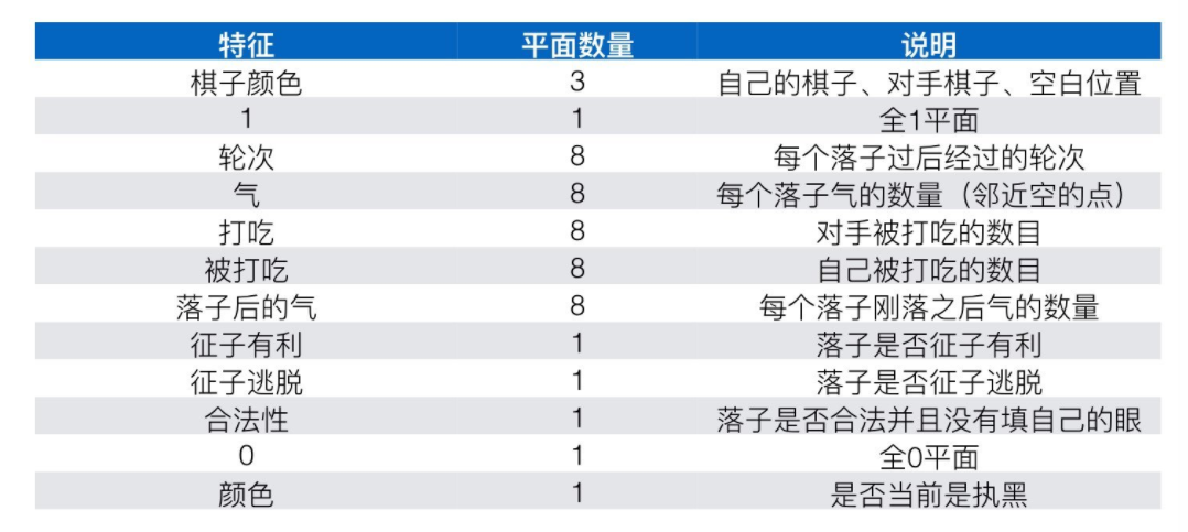
All features were computed relative to the current colour to play; for example, the stone colour at each intersection was represented as either player or opponent rather than black or white (所有的特征都是相对于当前下子的人来说，我们用的是player or opponent，而不是用黑白子).Each integer feature value is split into multiple 19 × 19 planes of binary values (one-hot encoding). For example, separate binary feature planes are used to represent whether an intersection has 1 liberty, 2 liberties,…, ≥8 liberties. (整数特征全部转换为one hot编码，比如气数，用8个平面分别表示不同的数值)，完整的输入特征如下：

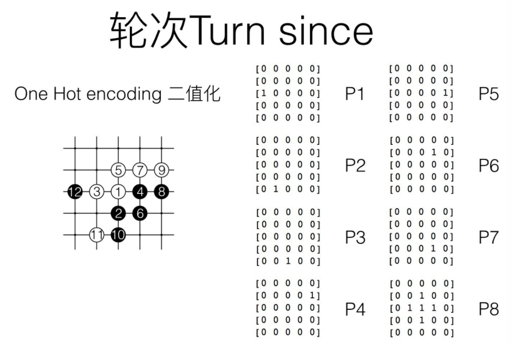
关于其中的轮次解释一下（就是最近7次的落子位置和第8次前的棋盘状态，下棋是一个连续的动作，最近几次下子对本次下子很有作用）：

Neural network architecture

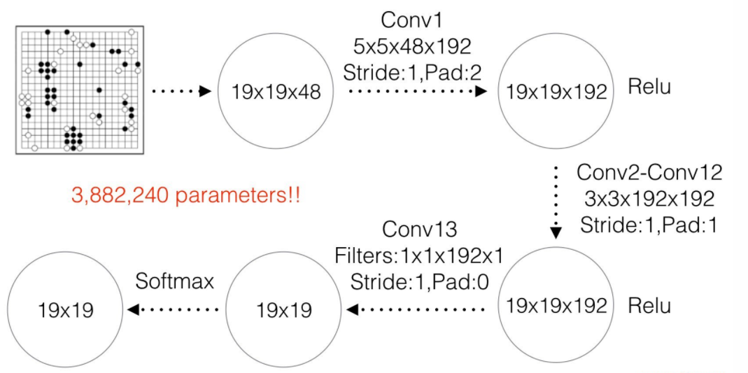
The input to the value network is also a 19 × 19 × 48 image stack, with an additional binary feature plane describing the current colour to play. Hidden layers 2 to 11 are identical to the policy network, hidden layer 12 is an additional convolution layer, hidden layer 13 convolves 1 filter of kernel size 1 × 1 with stride 1, and hidden layer 14 is a fully connected linear layer with 256 rectifier units. The output layer is a fully connected linear layer with a single tanh unit.

Summary

再次引用结构总图：

其中快速下子网络是用来评估位置价值的时候一种方式（全部按照此策略下完，直接返回结果），而SL网络一方面用来作为RL网络的初始参数，一方面用于value 网络前面部分的棋盘的生成；RL网络真的就只是为了得到value 网络，其后面的策略全部采用RL policy；value 网络结合fast rollout network一起评价action value。而MCTS将这个结构搭建在一起，通过选择访问次数最多的方法实现了更强的鲁棒性，而很多次的蒙特卡洛模拟正是访问次数生成的关键。总的来说，整体的思想就是通过策略网络集中搜索方向，而value网络用语尽早截断搜索，后面的估计全部用value网络实现。

下面是论文全文：Mastering the game of Go with deep neural networks and tree search