FFT

FFT is a methods for computing the DFT efficiently. In view of the importance of the DFT in various digital signal processing applications, such as linear filtering(线性滤波), correlation analysis（相关分析）, and spectrum analysis（谱分析）, its efficient computation is a topic that has received considerable attention by many mathematicians, engineers, and applied scientists.

DFT

Basically, the computational problem for the DFT is to compute the sequence {X(k)} of N complex-valued numbers given another sequence of data {x(n)} of length N (sample length), according to the formula:

$X(k)=\sum _{n=0}^{N-1} x(n) W_N^{\text{kn}}, 0\leq k\leq N-1\\ W_N=e^{-\frac{\text{j2$\pi $}}{N}}$

and $W_n^k$ for k=0,1,…,N-1 are called the $N_{th}$ roots of unity. They’re called this because, in complex arithmetic, $(W_N^k)^N=1$ for all k. They are vertices(顶点) of a regular polygon inscribed in the unit circle of complex plane, with one vertex at (1,0). Below are roots of unity for N=2,N=4 and N=8, graphed in the complex plane.

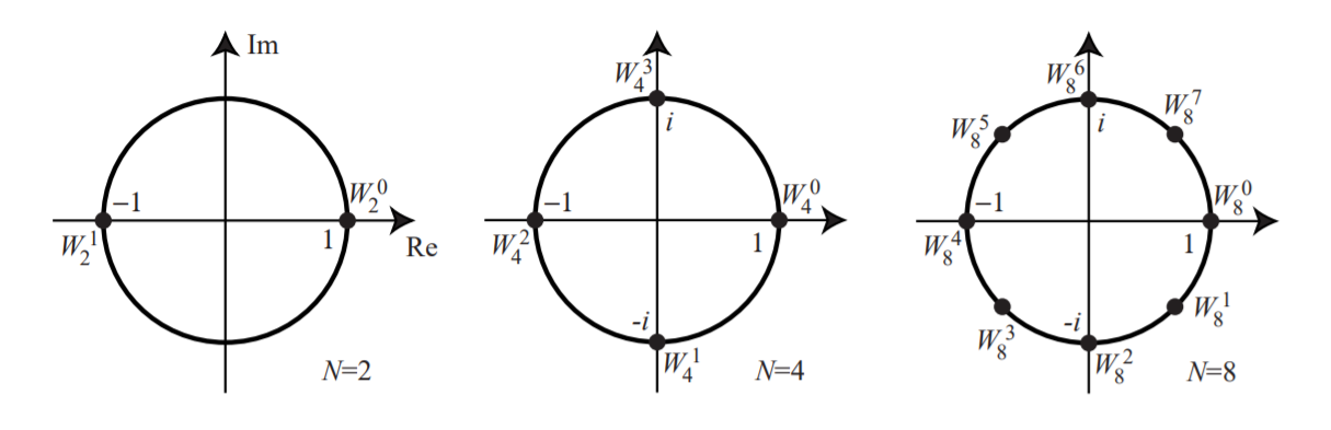
Powers of roots of unity are periodic with period N.

The sequence $A_k$ is the discrete Fourier transform of sequence $a_n$. Each is a sequence of N complex numbers. The sequence $a_n$ is the inverse discrete Fourier transform of sequence $A_K$ . The formula of the inverse DFT is:

$a_n=\frac{\sum _{k=0}^{N-1} A_k W_N^{-\text{kn}}}{N}$

Direct computation of the DFT is basically inefficient primarily because it does not exploit the symmetry and periodicity properties of the phase factor $W_n$. In particular, these two properties are : Symmetry property $W_N^{k+\frac{N}{2}}=-W_N^k$ ,Periodic property $W_N^{k+N}=W_N^k$ . Then FFT is come into our eyes.

Note the N-point DFT can be expressed in terms of the DFT’s of the decimated sequences as follows:

$\begin{aligned}X(k)&=\sum _{n=0}^{N-1} x(n) W_N^{\text{kn}}\\ &=\sum _{x\in \text{even}}x(n)W_N^{\text{kn}}+\sum _{x\in \text{odd}}x(n)W_N^{\text{kn}}\\ &=\sum _{m=0}^{\frac{N}{2}-1} x(2 m) W_N^{2 \text{mk}}+\sum _{m=0}^{\frac{N}{2}-1} x(2 m+1) W_N^{k (2 m+1)}\end{aligned},0\leq k\leq N-1$

But $W_N^2=e^{-\frac{2 \text{j2$\pi $}}{N}}=e^{-\frac{\text{j2$\pi $}}{0.5 N}}=W_{\frac{N}{2}}$ ,with this substitution, the equation can be expressed as:

$\begin{aligned}X(k)&=\sum _{m=0}^{\frac{N}{2}-1} x(2 m)W_{\frac{N}{2}}^{\text{km}}+W_N^k \left(\sum _{m=0}^{\frac{N}{2}-1} x(2 m+1)W_{\frac{N}{2}}^{\text{km}}\right)\\ &=F_1 (k)+F_2 (k) W_N^k\end{aligned}$

Since $F_1(k)$ and $F_2(k)$ are periodic, with period N/2, we have $F_1(k+N/2)=F_1(k)$ and $F_2(k+N/2)=F_2(k)$. In addition, the factor $W_n^{k+N/2}=-W_n^k$. Hence the equation may be expressed as:

$\text{X(k)}=F_1 (k)+F_2 (k) W_N^k,k=0,1,\text{...},\frac{N}{2}-1\\ \text{X(k+N/2)}=F_1 (k)-F_2 (k) W_N^k,k=0,1,\text{...},\frac{N}{2}-1\\$

where $F_1(k)$ and $F_2(k)$ are $N/2$ point DFTs, we can use the FFT method again and again until a two point DFTs.

In conclusion, the FFT algorithm decomposes the DFT into $log_2(N)$ Stages, each of which consists of N/2 butterfly computations. Each butterfly takes two complex numbers p and q and computes from them two numbers, $p+\alpha q$ and $p-\alpha q$ , where $ \alpha$ is a complex number. Below is a diagram of butterfly operation:

use the diagram we can draw the flow chart of FFT, here is a 8-point FFT flow chart:

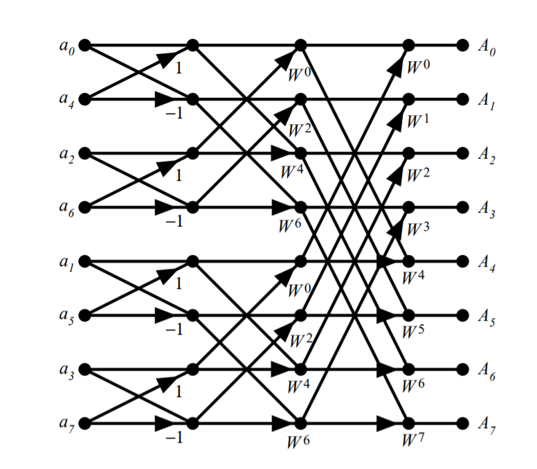
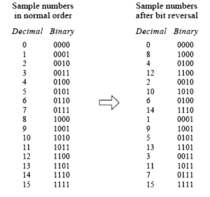
It’s obviously the inputs aren’t in the normal order. In order to see this more clearly, following is a 16-point FFT:

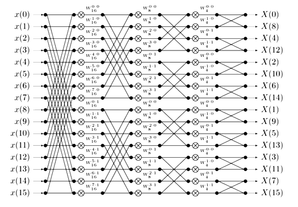
we can follow the decomposition process as the figure:

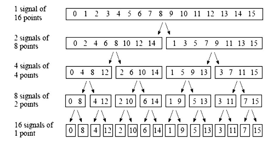
If we use a binary tree, it easy to find the sample numbers $n_j$ is the bit-reversal of j.

Computational complexity of FFT

The FFT is a fast algorithm for computing the DFT. If we take the 2-point DFT and 4-point DFT and generalize them to 8-point,16-point,…,$2^r$-point, we get the FFT algorithm. To compute the DFT of N-point sequence using original DFT would take $O(n^2)$ multiplies and adds. The FFT algorithm computes the DFT using $O(n logN)$ multiplies and adds.

Discrete Fourier Transform - Simple Step by Step:

The FFT Algorithm - Simple Step by Step:

Code FFT In MATLAB

After the discussion above, it is easy to code the FFT function:

function [X] = FastFourierTransform(x)
%将x进行快速傅里叶变换
N=numel(x);         %number of array elements
if(mod(N,2)==0)     %可以利用FFT的部分
    if N>=4         %采用奇偶分开的方法
        F1=FastFourierTransform(x(1:2:end));	%奇数部分
        F2=FastFourierTransform(x(2:2:end));    %偶数部分
        Wn=exp(-1i*2*pi*((0:N/2-1)')/N);
        Butterdiff=Wn.*F2;  %因为MATLAB下标从1开始，这里用F2
        X = [(F1 + Butterdiff);(F1 -Butterdiff)];
    else
        X=[1 1;1 -1]*x;     %2-point ft
    end
else        %考虑到x不一定是2的幂，所以不能拆分的部分采用基本的DFT
    X=FourierTransform(x);
end
end

function [X] = FourierTransform(x)
%将x进行傅里叶变换
N=numel(x);         %number of array elements
X=zeros(N,1);       %预先分配内存
Wn=exp(-1i*2*pi*((0:N-1)')/N);
for k=1:N
    X(k)=sum(x.*(Wn.^(k-1)));   %k should start at 0,so use k-1
end
end

You can see, in the algorithm, the input may not always in the shape of $2^m$ , so I use half FFT and half DFT when this happens. In order to compare the efficiency of the function, we compare it with the build in MATLAB function, here is the result:

N=2424;              %Not 2^m
data = rand(N, 1);   % Test data
t1=clock;
X1=FastFourierTransform(data);
t2=clock;
X2=fft(data);
t3=clock;
disp('FastFourierTransform cost: ');
disp(etime(t2,t1));
disp('FFT cost ');
disp(etime(t3,t2));
disp('differ:');
disp(norm(X1-X2,inf));

%the result is:
>> TestEfficient
FastFourierTransform cost: 
    0.1830

FFT cost 
     0

differ:
   1.8622e-11

%change N=4096
>> TestEfficient
FastFourierTransform cost: 
    0.0650

FFT cost 
    0.0020

differ:
   3.7974e-14

Obviously, if length of data is shaped $2^m$ , the speed is faster, but there is still a big gap between self-define function and MATLAB build in function. I think the reason is that MATLAB build in function use C language, which is fast than MATLAB language.

Applications

The FFT used in many fields, here list out some usage:

Filtering using FFT in Images

Removing noise from audio using FFT

Fast large integer and polynomial multiplication

Solving difference equations

Fast Chebyshev approximation

Fast large integer and polynomial multiplication

The function of FFT is similar, if it is more convenient to analysis in frequency domain, then use FFT first, then operate the signal in frequency domain, transfer to time domain after that.

Here I will introduce a example I’m interested in: Analyzing Cyclical Data

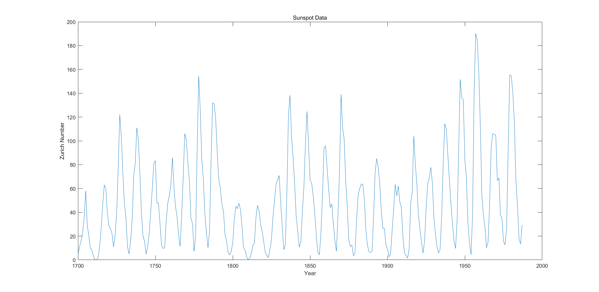
For almost 300 years, astronomers have tabulated the number and size of sunspots(太阳黑子) using the Zurich sunspot relative number. Plot the Zurich number over approximately the years 1700 to 2000. We will use FFT to find it’s feature.

load sunspot.dat 		%first load data
year = sunspot(:,1);
relNums = sunspot(:,2);
plot(year,relNums)
xlabel('Year')
ylabel('Zurich Number')
title('Sunspot Data')	%plot the sunspot number relation with time

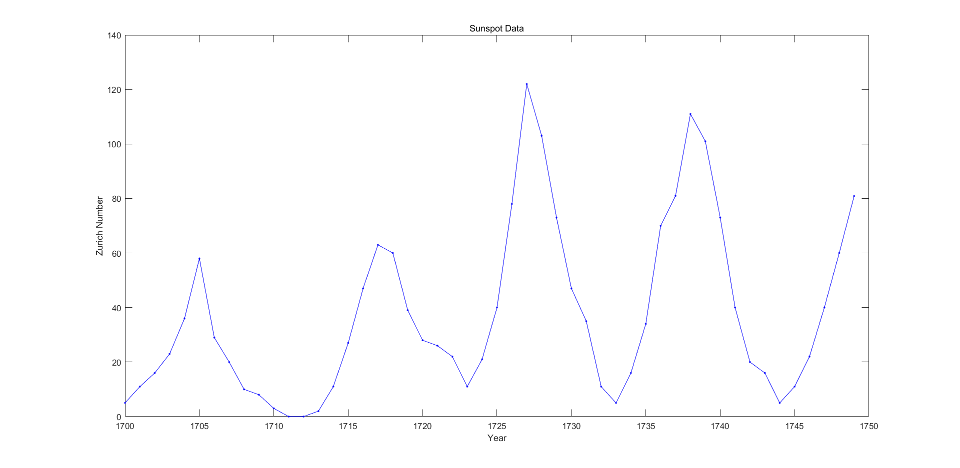
%To take a closer look at the cyclical nature of sunspot activity, plot the first 50 years of data.
plot(year(1:50),relNums(1:50),'b.-');
xlabel('Year')
ylabel('Zurich Number')
title('Sunspot Data')

y = fft(relNums);				%use FFT to identifies frequency components in data
y(1) = [];
n = length(y);
power = abs(y(1:floor(n/2))).^2; % power of first half of transform data
maxfreq = 1/2;                   % maximum frequency, 根据采样定理，只有一半
freq = (1:n/2)/(n/2)*maxfreq;    % equally spaced frequency grid
plot(freq,power)
xlabel('Cycles/Year')
ylabel('Power')

period = 1./freq;				%in order to see the period more clearly
plot(period,power);
xlim([0 50]); 					%zoom in on max power
xlabel('Years/Cycle')
ylabel('Power')

the result is as follow:

sunspot Data in 300 years:

sunspot data in 50 years:

sunspot power with period:

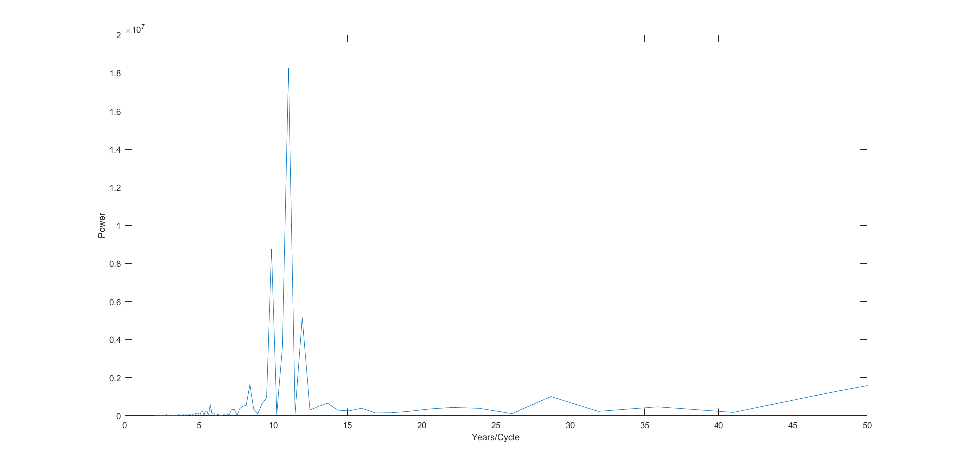
The plot reveals that sunspot activity peaks about once every 11 years.

Here also give a code in de-noise, but this is simple so I won’t do experiment anymore (the process is easy to understand)

fft_values = fft(samples); 		%samples is the origanl signal
mean_value = mean(abs(fft));	%Get the mean value
threshold  = 1.1*mean_value; 	%calculate a threshold, coeficient can be changed
fft_values[abs(fft_values) < threshold] = 0; 
%denoise 噪声通常都是相对较小一点的（这个方法只适合去除噪声相对较小的情况）
filtered_samples = ifft(fft_values);%得到降噪后的信号

Reference

http://www.cmlab.csie.ntu.edu.tw/cml/dsp/training/coding/transform/fft.html
https://en.wikipedia.org/wiki/Fast_Fourier_transform
https://cn.mathworks.com/help/matlab/examples/using-fft.html
Heckbert P. Fourier Transforms and the Fast Fourier Transform (FFT) Algorithm[J]. Comp. Graph, 1995, 2: 15-463.

Blog

FFT

DFT

FFT

Computational complexity of FFT

Code FFT In MATLAB

Applications

Reference

Search

Table of Contents

FFT

DFT

FFT

Computational complexity of FFT

Recommend Video of FFT

Code FFT In MATLAB

Applications

Reference

Search

Table of Contents